Day 3: Arrays, Linked Lists, and Intro to Abstract Datatypes
Homework Debrief
How did the assignment go? Do a quick check-in with those around you and see if you can surface 1-2 questions that are still unresolved for you.
Meeting Our First Data Structures
Today we’re going to meet our first data structures of the semester: the array and the linked list. We’ll talk about tradeoffs in terms of runtime of various operations on these data structures. We’ll also introduce the concept of abstract data types (ADTs) as a tool for separating the implementation of a data structure from the operations it supports.
Arrays
As we mentioned on day one, data structures represent different approaches to organizing data in some digital storage system. In this course, we’re going to learn about a bunch of different data structures (e.g., linked lists, arrays, binary trees, graphs, etc.). To help us wrap our minds around the big ideas of data structures, let’s consider a very useful data structure: an array.
Depending on your programming background, perhaps you haven’t encountered an array yet. An array is an ordered collection of values (usually of a particular type). Arrays are typically implemented in a computer using a contiguous block of memory (e.g., stored in the computer’s RAM).
When we create an array, we have to specify the capacity that we’d like our array to have (that is the size that we’d like to reserve for our array in the computer’s memory). Upon requesting an array of a particular size, we will be allocated a contiguous region in the computer’s memory to store our values. We can assume that requesting and being assigned a region in memory is relatively efficient (think of this as taking a constant number of operations). Further, we can assume that we can efficiently write and read values from an array (think of these as taking a constant number of operations).
Time Complexity of Various Array Operations
As stated above, for these operations we can assume that requesting new memory, reading a single value, and writing a single value for our array takes a constant number of operations.
Exercise 1: Suppose you have an array with $M$ elements and there is space for $C$ elements in the block of memory allocated to your array (with $M < C$). Assume that the $M$ elements are stored such that they occupy the first $M$ slots of memory allocated to the array. How many steps would it take to add a new element to the end of your array? Going back to our discussion of order-of-growth, what is the running time of this operation in terms of $\Theta$?
Exercise 2: Now, suppose you’d like to add an element to the beginning of your array. If there are currently $M$ elements in your array, how many operations would it take to add an element to the beginning of the array? What is $\Theta$ for this operation?
Exercise 3: Now, suppose you want to add an element ot the end of your array but the number of elements stored in the array is equal to the current capacity $M = C$. How many operations would it take to perform the following steps: request a size $M+1$ block of memory, copy the first $M$ elements to the new memory block, and then add the new element to the array? Suppose you start $M = C = 1$ (an empty array with no capacity). How many operations would it take to add $N$ elements to the end of this array if you added them one-by-one? Determine $\Theta$ of the time complexity of adding these $N$ elements.
Exercise 4: Similar to the previous problem, suppose you want to add $N$ elements to the end of an array in a one-by-one fashion. Let’s see if we can do better than we did in problem 3. Instead of adding 1 unit of capacity every time we run out of space in our array, we’re going to multiply our capacity by a factor of 2 (e.g., starting we start with capacity 1, then go to capacity 2, then capacity 4, and so on). How many operations would it take to add $N$ elements to the end of this array if you added them one-by-one and follow the strategy of doubling the capacity of the array each time you run out of space (for simplicity you can assume that $N$ is a power of 2)? Determine $\Theta$ of the time complexity of adding these $N$ elements in this fashion.
Linked Lists
Next, we’re going to learn about a data structure that excels at many of the operations that arrays are slow at and lags behind in areas where arrays are fast. This data structure is the linked list.
A linked list is another way to represent an ordered collection of values. Instead of storing our collection in a contiguous block of memory, instead we store data in nodes that each contain a value and a reference to both the next node and the previous node in our list (this sort of linked list is called a doubly linked list). In addition to these nodes, we also maintain a reference to the first element (or the head of the linked list) and a reference to the last element (or tail of the linked list). Let’s draw a picture of what this looks like on the board together.
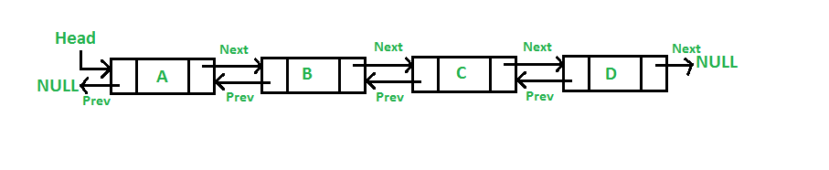 figure from geeksforgeeks
Now let’s do some problems to understand the time complexity of various operations on our linked list. For the purposes of these exercises, let’s assume that we can request memory to store a new linked list node in constant time ($\Theta(1)$).
Exercise 5: With folks around you, determine the time complexity ($\Theta$) of each of these operations on a linked list. For each of these, make a list of the steps you’d have to do in order to accomplish each of these operations. Count up the number of operations. What is $\Theta$ for this count?
- Add an element to the beginning of the list
- Delete an element from the beginning of the list
- Add an element to the back of the list
- Delete an element from the back of the list
- Print out the middle element of the list
Exercise 6: A singly linked list is a linked list where each node only has a reference to the next element in the list. In such a list, would the $\Theta$ of any of these operations in problem 5 be different? If so, which would be different and what are their new $\Theta$ running times?s
Abstract Data Types
A common strategy for managing complexity in software is to separate the details of how a piece of software works (the implementation) from the functions that the software performs (the interface). You may have seen this when you encountered object-oriented programming in Software Design. When you created Python classes, you would define methods on those classes that could then be called to perform some operation. The details of how these operations were carried out, were opaque to the caller (e.g., another class in our program). In our study of data structures, we will make a similar distinction between the operations that a data type performs, and the specific underlying data structure that is used to implement this data type.
We call the specification of a set of operations (or semantics) for a data type an Abstract Data Type (or ADT). For instance, we might specify an ADT to represent an ordered collection with the following operations:
- Insert at a new element at position $i$
- Delete element at position $i$
- Access element at position $i$
- Append an element to the end of the list
- etc.
The actual implementation of this abstract data type (called a concrete data type) could use a linked list or an array (or something more exotic) as the underlying data structure. Determining what concrete data type to use to implement a specific ADT will depend on the operations are most important for your application (you’ll want to make those fast). Perhaps, you could even create different implementations of the same ADT for different use cases (e.g., if you care about accessing elements quickly or adding new elements).
Exercise 7: For example, the Python tutorial on lists states that while accessing elements in the list, appending an element ot the end of the list, or removing an element from the end fo the list is fast, adding or deleting an element at the beginning of the list is slow. Based on what you worked out earlier in class, what underlying concrete data structure do you think Python uses for its list class? Do some research to see if you are right.
Stacks vs. Queues
In the next assignment, you will be implementing both a stack and a queue. Each of these data structures will be built on top of a linked list, but stacks and queues will differ with respect to some of their behaviors. Specifically, stacks use what is called a LIFO (last in first out) ordering whereas queues utilize a FIFO ordering (first in first out). You’ll get a bunch of practice using your stacks and queues to solve problems in the assignment, but you might also want to check out this short article comparing the two data structures.
Kotlin Interfaces
Let’s learn about Kotlin interfaces and why they are a useful way to define abstract datatypes.
Let’s say we want to design a simple 2D geometry library. We may want to define the abstract datatype shape as one that supports a set of operations. Perhaps each shape can compute its area and perimeter. We can formalize this idea using a Kotlin interface.
interface Shape {
    fun area(): Double
    fun perimeter(): Double
}
This interface is like a contract that any class that implement the Shape interface must fulfill. For example, we could create a class called circle in the following way.
class Circle(private val radius: Double) : Shape {
    override fun area(): Double {
        return Math.PI * radius * radius
    }
    override fun perimeter(): Double {
        return 2.0 * Math.PI * radius
    }
}
We might define a rectangle in the following way.
class Rectangle(private val width: Double,
                private val height: Double) : Shape {
    override fun area(): Double {
        return width*height
    }
    override fun perimeter(): Double {
        return 2.0 * (width + height)
    }
}
The nice thing is that we can write functions that operate on any class that implements this particular interface.
fun totalArea(shapes: List<Shape>): Double {
    return shapes.sumOf { it.area() }
}
This lets us do things like:
fun main() {
    println(
        totalArea(listOf(Circle(5.0),
                         Rectangle(2.0, 4.0)))
    )
}